Schedule Variance Formula: What SV Measures and Where It Fails

Schedule variance is SV = EV − PV: earned value minus planned value at a point in time. Negative means behind plan. The result is in currency, not days, and it has a property most explanations omit — as a project finishes, earned value converges on planned value, so SV approaches zero and the schedule performance index approaches 1.0 even when the project is late.
Key takeaways
- SV = EV − PV and SPI = EV ÷ PV. Both are computed from budgeted values, so both are expressed in money.
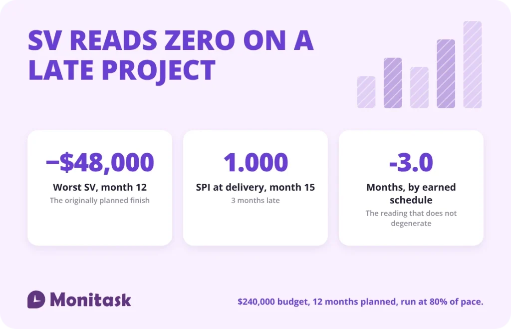
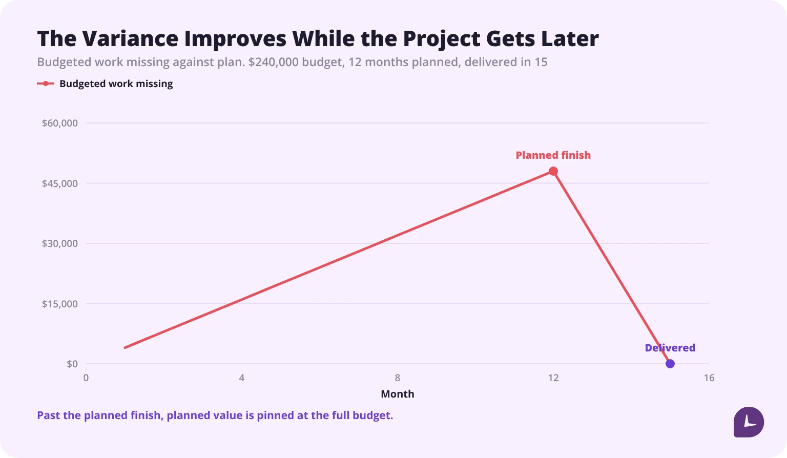
- On a project running at 80% of planned pace, SV peaks at −$48,000 in month 12 and falls to $0 by month 15 — as the delay grows.
- SPI on that same project reads 1.000 at delivery, 3 months late.
- Earned schedule gives the same project SV(t) = −3.0 months and SPI(t) = 0.800, which do not degenerate.
- On a realistic S-curve baseline, SPI is wrong at every point of the project, not just the last third — reading 0.652 when the true pace is 0.80 and 0.905 by the planned finish.
- Identical dollar variance on two tasks produces a 20-day slip or none at all, depending on float.
What is the schedule variance formula?
SV = EV − PV
| Term | Full name | Older notation | What it is |
|---|---|---|---|
| PV | Planned value | BCWS — budgeted cost of work scheduled | The budgeted value of the work the plan says should be complete by this date |
| EV | Earned value | BCWP — budgeted cost of work performed | The budgeted value of the work actually complete by this date |
| BAC | Budget at completion | — | The approved total budget for the whole project |
| AC | Actual cost | ACWP — actual cost of work performed | What has actually been spent; not used in SV |
PV is a time-phased figure, not the whole budget. BCWS is the budgeted cost of work scheduled up to the assessment date — confusing it with BAC is the most common error in the older notation, and it makes the formula return nonsense.
Reading the sign:
| Result | Meaning |
|---|---|
| SV < 0 | Less work complete than planned — behind plan |
| SV > 0 | More work complete than planned — ahead of plan |
| SV = 0 | Earned value equals planned value — on plan |
SV = 0 means on plan. It does not mean all the work is finished, and as the next sections show, it does not reliably mean on schedule either.
Both inputs depend on a percent-complete assessment, so the variance is only as good as that assessment. A percent complete measured by effort spent rather than work delivered will produce an SV that looks healthier than the project is.
Why is schedule variance measured in money?
Because both inputs are budgeted values. PV and EV are expressed in the currency of the budget, so their difference is too. The quantity called schedule variance is denominated in dollars, and that is the long-standing objection to it.
The point is made directly in the Project Management Institute’s own library. In “The practical calculation of schedule variance in terms of schedule,” presented at PMI Global Congress 2008, Warburton and Kanabar write: “A major criticism of the standard EVM is that the schedule variance is measured in cost units, not time.”
There is a practical reason for the design. Expressing variance in money lets different kinds of work be added together: writing, testing and procurement have no common physical unit, but each has a budgeted value, so a single figure can summarise the whole project. That is a real benefit and it is why the measure is built this way.
The cost of the design is that the number cannot be read as a date. A variance of −$48,000 says how much budgeted work is missing, not how many days behind the project is, and converting between the two requires an extra assumption covered further down.
Does schedule variance reach zero on a late project?
Yes, and that is the most important property of the formula. Because both EV and PV are capped at the budget at completion, they converge as the work finishes — so the variance between them shrinks while the delay grows.
Take a project with a budget of $240,000 and a planned duration of 12 months, planned linearly at $20,000 a month. It runs at 80% of planned pace throughout, earning $16,000 a month, and therefore finishes in 15 months — 3 months late.
| Month | PV | EV | SV | SPI |
|---|---|---|---|---|
| 6 | $120,000 | $96,000 | −$24,000 | 0.800 |
| 9 | $180,000 | $144,000 | −$36,000 | 0.800 |
| 12 | $240,000 | $192,000 | −$48,000 | 0.800 |
| 13 | $240,000 | $208,000 | −$32,000 | 0.867 |
| 14 | $240,000 | $224,000 | −$16,000 | 0.933 |
| 15 | $240,000 | $240,000 | $0 | 1.000 |
At month 15 the project is delivered 3 months late — a 25% schedule overrun — and the schedule variance is $0 with an SPI of 1.000. Both metrics report a project exactly on schedule.
This is not a quirk of the worked example. Lipke, who proposed the time-based alternative described below, states it as a general property: “Schedule Variance must converge to 0.0 at project completion, while the Schedule Performance Index concludes at 1.0” — and it happens “without fail for every project finishing late”.
Notice the shape. The variance is at its worst in month 12, the originally planned finish date, and then improves every month while the project gets later. After month 12, PV is pinned at the full budget because the plan says everything should already be done, so every additional month of work closes the gap. The metric is not malfunctioning; it is doing exactly what the formula specifies, and the formula’s answer stops corresponding to the question.
When does SPI stop being useful?
On a straight-line plan, in the last phase. On a realistic plan, everywhere.
The straight-line case
| Month | SPI | SPI(t), time-based | Divergence |
|---|---|---|---|
| 12 | 0.800 | 0.800 | 0.000 |
| 13 | 0.867 | 0.800 | 0.067 |
| 14 | 0.933 | 0.800 | 0.133 |
| 15 | 1.000 | 0.800 | 0.200 |
The PMI paper records the same effect, though it is worth being precise about whose view it is. The paper reports as a criticism — made by Corovic (2007), Fleming and Koppelman, Lipke (2003, 2004), Henderson (2004), and Vandevoorde and Vanhoucke (2006) — that since SPI approaches 1.0 at the end of a project, it is “not useful over the last third of the project”. Warburton and Kanabar then partly disagree, saying one of their own exhibits “somewhat blunts this criticism”. So it is a widely held objection rather than a settled finding, and the paper usually cited for it is in fact arguing against it.
What a real baseline does
The table above uses a linear plan and a constant pace, so SPI holds at 0.80 right up to the planned finish and only misleads from month 13. Real baselines are S-curves: planned value accrues slowly at first, quickly through the middle, and slowly again at the end. Running the identical project against an S-curve of the same budget and the same 80% pace gives a different and worse picture.
| Month | SPI, straight line | SPI, S-curve | SPI(t), either |
|---|---|---|---|
| 3 | — | 0.652 | 0.800 |
| 6 | 0.800 | 0.691 | 0.800 |
| 9 | 0.800 | 0.767 | 0.800 |
| 12 | 0.800 | 0.905 | 0.800 |
| 13 | 0.867 | 0.957 | 0.800 |
| 14 | 0.933 | 0.989 | 0.800 |
| 15 | 1.000 | 1.000 | 0.800 |
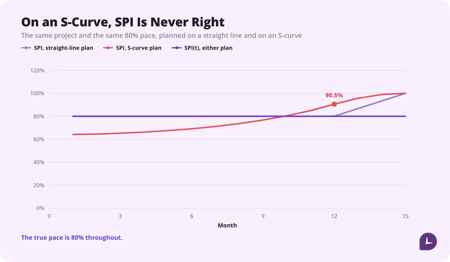
On the S-curve, classic SPI is never right. It reads 0.652 at month 3, understating a team that is actually working at 0.80, because the plan expects a fast middle the team has not reached. It crosses the true pace around month 9 and then overstates: by the planned finish it reads 0.905, which is 0.105 more optimistic than the straight-line model gives at the same moment. The degeneration does not begin after the planned finish. It has been under way since roughly the midpoint.
The S-curve also moves the peak. On a straight line the variance is worst at month 12; on the S-curve it is worst at month 9 — −$47,771 — and has already shrunk by 52% by the planned finish. A manager watching SV alone would see the project apparently recovering for a quarter of its life while it was in fact running at a constant 80% throughout.
The PMI paper’s own conclusion is about exactly this trap: “An inexperienced project manager might interpret this to mean that while the project did not start well, the rise in CPI(t) indicates that improvements have been made. In fact, nothing has changed, and the project has an over-run in both cost and schedule”. Its warning is that “these warning signs are time-dependent, and must be interpreted with great care”.
The practical consequence is for forecasting. A forecast duration derived by dividing planned duration by SPI inherits the same flaw: as SPI drifts up toward 1.0, the forecast drifts back toward the original plan, and the forecast becomes most optimistic exactly when the project is latest, and any dashboard built on that forecast inherits it too.
How do you measure schedule variance in time?
By asking a different question: not how much value is missing, but when the value actually earned was supposed to have been earned. That date is the earned schedule, and the variance is the gap between it and today. The measure is Walt Lipke’s, set out in “Schedule is Different” in The Measurable News in 2003.
| Term | Formula | Units |
|---|---|---|
| ES — earned schedule | The point on the baseline at which the current EV was planned to be achieved | Time |
| AT — actual time | Elapsed time to the assessment date | Time |
| SV(t) | ES − AT | Time |
| SPI(t) | ES ÷ AT | Ratio |
On the project above at month 15, EV is $240,000. The plan earned $20,000 a month, so that value was scheduled to be complete at month 12. ES is therefore 12.0 months while AT is 15.
| Classic measure | Earned schedule | |
|---|---|---|
| Variance | SV = $0 | SV(t) = −3.0 months |
| Index | SPI = 1.000 | SPI(t) = 0.800 |
| What it reports | No variance | 3 months late, running at 80% pace |
| What was actually true | 3 months late, running at 80% pace | — |
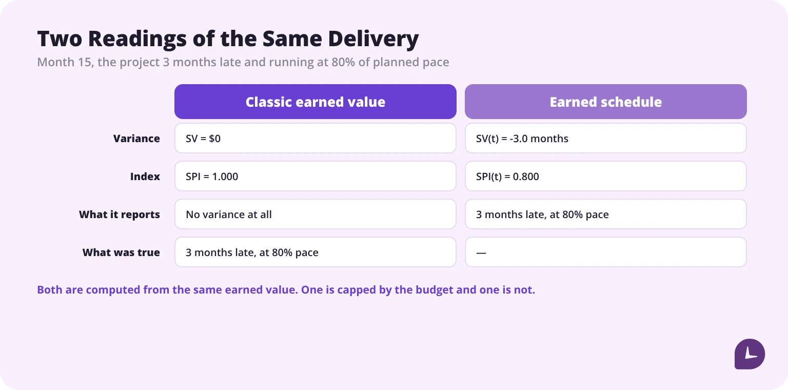
SPI(t) reads 0.80 at every assessment point in the project — month 6, month 12 and month 15 alike — because it compares time earned with time spent, and neither is capped by the budget. It gives the same answer at the end as at the start, which is what a performance index is for. It also reads 0.80 on the S-curve plan, at every point, because it does not care what shape the baseline is.
Two cautions. The earned schedule reading depends on being able to locate the current EV on the baseline, which is straightforward with a linear or monotonic plan and less so with a plan that has flat sections. And a time-based reading is a diagnostic complement to earned value rather than a drop-in replacement for it — it still inherits whatever error sits in the percent-complete assessment that produced EV in the first place, which is why it is worth knowing where the underlying hours came from. Time tracking is the record that assessment should be built on.
> A notation trap worth knowing about. The PMI paper cited earlier also uses the symbols SV(t) and SPI(t), but it means something else by them: the ordinary cost-unit measures written as functions of time. It does not state the earned schedule equations and does not cite Lipke in its derivations. If you are reading across sources, check which SV(t) an author means before comparing figures.
Does SV tell you whether you will be late?
No. Schedule variance has no knowledge of the network, so it cannot distinguish work that drives the finish date from work that does not.
Two tasks, each with an identical variance of −$18,000 and a planned burn of $900 a day:
| Task | SV | Equivalent days of work | Float available | Effect on the project finish date |
|---|---|---|---|---|
| A, on the critical path | −$18,000 | 20.0 days | 0 days | 20.0 days late |
| B, with float | −$18,000 | 20.0 days | 20 days | No slip |
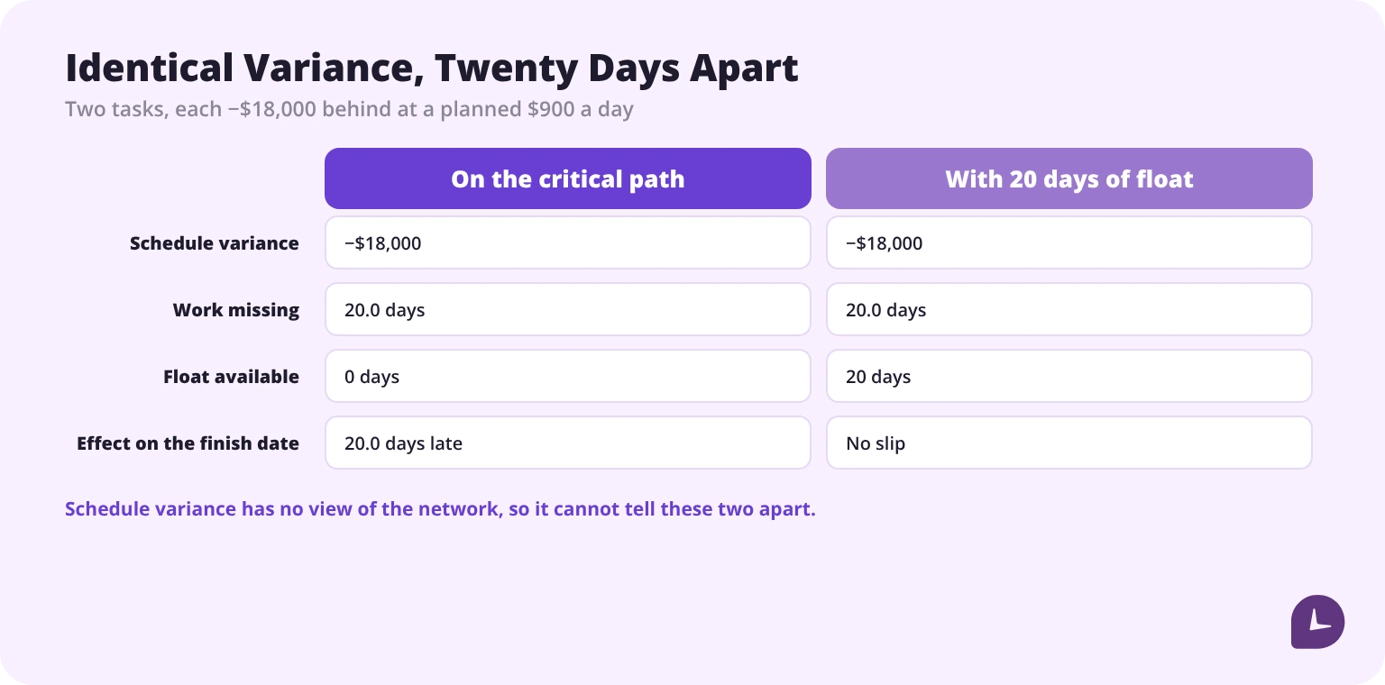
The dollar figures are the same. The schedule consequences are twenty days apart. A project showing a large negative SV concentrated in float-rich work can still finish on time, and a project showing a small negative SV sitting on the critical path can be badly late.
This is why schedule variance belongs next to a critical path analysis rather than instead of one. The variance tells you how much budgeted work is missing; the network tells you whether that work matters to the date. Neither answers the other’s question, and neither says anything about whether the people needed for that work are available — which is a resource allocation question.
How do you convert schedule variance into days?
Divide the variance by the planned burn rate for the period:
Time variance = SV ÷ planned value rate
The formula is Anbari’s, from “Earned value project management method and extensions” in the Project Management Journal in 2003. On the example project, SV of −$48,000 at month 12 against a planned rate of $20,000 a month gives −2.4 months. That matches the time-based variance for month 12 exactly, which is not a coincidence: where the planned rate is constant, the simple conversion and earned schedule are the same calculation.
The conversion holds only while that rate is constant, and the PMI paper quotes it in order to attack precisely that assumption. It notes that the PV rate “the PV Rate is calculated as the total budget divided by the total schedule (both at completion), and is assumed to be constant over the life of the project”, that dividing by it means “When one divides the current SV (at time, t) by the PV Rate, one is assuming that the average PV Rate applies for all time.”, and concludes: “The assumption that the parameters are independent of time is manifestly not true.”
Once the plan is an S-curve, the rate differs at every point, so there is no single divisor: using an average rate understates the variance during the steep middle of the plan and overstates it at the ends. That boundary is precisely where the simple conversion stops working and earned schedule begins — and it is the same boundary that makes classic SPI misread an S-curve from the midpoint onward.
Two practical rules follow. Use the conversion for a short-horizon reading on a plan that is locally linear, and quote the divisor you used alongside the result. And never convert on a project past its planned finish date, because the numerator is already collapsing toward zero for the reasons set out above.
Should SV be calculated per task or per project?
Both, for different purposes.
| Level | What it answers | Limitation |
|---|---|---|
| Task or work package | Where the variance originated, and whether that work has float | Too granular to summarise status; noisy on short tasks |
| Control account or phase | Which part of the project is behind | Hides offsetting variances inside it |
| Project | Total budgeted work missing against plan | Says nothing about the finish date; degenerates near completion |
The project-level figure is the one reported and the task-level figure is the one acted on. Aggregating conceals the two things that determine consequence: a project total of −$18,000 could be one critical task twenty days behind or nine non-critical tasks each slightly behind, and only the breakdown distinguishes them. Tracking time by project and task is what makes the breakdown available.
A related trap is offsetting. Work running ahead in one area nets against work running behind in another, and the project SV reports the difference. Since work ahead of plan rarely pulls a finish date forward while work behind plan reliably pushes it back, the netted figure is systematically optimistic.
What does schedule variance not tell you?
| Question | Does SV answer it? |
|---|---|
| How much budgeted work is missing against plan? | Yes — this is what it measures |
| How many days behind is the project? | No, not without a rate conversion and its assumptions |
| Will the finish date slip? | No — it has no view of the critical path or float |
| Is the project over budget? | No — that is cost variance, which uses actual cost |
| Is the delay getting worse? | Not reliably — the figure shrinks after the planned finish date, and sooner than that on an S-curve |
| Where did the delay come from? | Only if calculated per work package |
| Is the percent complete correct? | No — it inherits whatever error is in that assessment |
| Is the remaining plan still achievable? | No — that needs a re-planned baseline, not a variance |
Earned value needs a defensible percent complete, and that starts with knowing where hours actually went by project and task.
See how workforce analytics works in Monitask
Sources
- Warburton, R. D. H., & Kanabar, V. (2008). “The practical calculation of schedule variance in terms of schedule.” Paper presented at PMI Global Congress 2008 — North America, Denver, CO. Project Management Institute. https://www.pmi.org/learning/library/practical-calculation-schedule-variance-7028
- Lipke, W. (2003). “Schedule is Different.” The Measurable News, March and Summer 2003. https://www.earnedschedule.com/Docs/Earned%20Schedule%20-%20schedule%20performance%20analysis%20from%20EVM%20measures.pdf
- Anbari, F. T. (2003). “Earned value project management method and extensions.” Project Management Journal, 34(4). Cited in Warburton & Kanabar (2008); see note below
All sources checked 22 October 2026. The Anbari conversion formula is quoted here as it appears in Warburton and Kanabar, who cite it in order to criticise the constant-rate assumption it depends on.
FAQ
Is schedule variance measured in time or money?
Money, despite the name. Both PV and EV are budgeted values, so their difference is denominated in the budget’s currency. The Project Management Institute’s own literature records this as a standing objection — “A major criticism of the standard EVM is that the schedule variance is measured in cost units, not time.”
What does a negative schedule variance mean?
That less budgeted work has been completed than the plan called for by that date. It quantifies the missing work in money. It does not by itself establish that the project will finish late, because it carries no information about which tasks the variance sits in or how much float they have.
Does schedule variance go to zero at the end of a project?
Yes, always — and that is its central weakness. Earned value and planned value are both capped at the budget at completion, so they converge as the work finishes. On a project running at 80% of planned pace, SV peaks at −$48,000 at the planned finish in month 12 and reads $0 at actual delivery in month 15, 3 months late.
Why does SPI approach 1.0 on a late project?
For the same reason. SPI is EV ÷ PV, and once the planned finish date passes, PV is pinned at the full budget while EV keeps rising toward it, so the ratio climbs to 1.0 at delivery regardless of how late that delivery is. On the example project SPI reads 0.80 through month 12, then 0.867, 0.933 and finally 1.000.
Does SPI only mislead in the last third of the project?
That is the usual criticism, but it is an artefact of assuming a straight-line baseline. Run the same project against an S-curve of the same budget and the same 80% pace and SPI is wrong throughout: 0.652 at month 3, understating the team, then crossing the true pace around month 9 and reading 0.905 by the planned finish. SPI(t) reads 0.80 at every point on both plans.
What is earned schedule?
A time-based reading of the same data, proposed by Walt Lipke in 2003. Earned schedule (ES) is the point on the baseline at which the currently earned value was planned to be achieved, and the variance is **SV(t) = ES − AT**, with **SPI(t) = ES ÷ AT**, where AT is elapsed time. On the example project at month 15, ES is 12.0 months, so SV(t) is −3.0 months and SPI(t) is 0.800 — the correct answers, where the classic measures report no variance at all.
How do you convert schedule variance from dollars into days?
Divide by the planned value rate for the period: **time variance = SV ÷ PV rate**, a conversion due to Anbari (2003). At −$48,000 against a planned $20,000 a month, that is −2.4 months. It only holds while the rate is constant, so it fails on an S-curve plan where the rate differs at every point, and it should never be applied past the planned finish date because the numerator is already collapsing.
Does schedule variance account for the critical path?
No. Two tasks with an identical variance of −$18,000, each equal to 20.0 days of planned work, produce a 20-day slip if the task is on the critical path and no slip at all if it has 20 days of float. Schedule variance has no view of the network, which is why it is read alongside a critical path analysis rather than in place of one.