

Workforce scheduling is the process of matching staffing to demand across time, within a labour budget and whatever rules apply to your workforce. Every article on the subject agrees on that definition, lists the same components, and then moves to software.
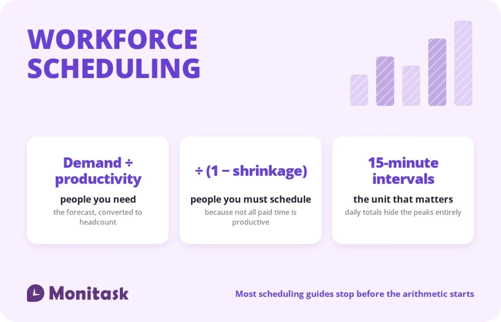
The part that decides whether a schedule works is quantitative, and three numbers do most of the work:
- Required staff = forecast demand ÷ productivity rate
- Scheduled hours = required productive hours ÷ (1 − shrinkage)
- Coverage is measured in intervals, not in daily totals
Miss the second one and you will be understaffed by roughly a quarter every single week while your headcount looks correct on paper. This guide covers the process briefly and the arithmetic properly.
Quick answer
| Question | Answer |
|---|---|
| What is workforce scheduling? | Assigning people to time periods so that staffing matches demand within a labour budget and the applicable rules |
| How do you size a shift? | Forecast demand, divide by productivity rate, then divide by one minus shrinkage |
| What is shrinkage? | The share of paid hours not spent on the primary work: breaks, training, meetings, absence. Commonly 25–35% |
| What interval should you plan in? | 15 or 30 minutes for demand-driven work; whole shifts only for fixed-coverage work |
| How far ahead should you publish? | 14 days, and it is legally required in eleven US jurisdictions |
| What should you measure? | Coverage variance, labour cost variance, overtime share, forecast accuracy |
Scheduling vs workforce management vs planning
Three terms, three time horizons.
| Workforce planning | Workforce scheduling | Workforce management | |
|---|---|---|---|
| Horizon | Quarters to years | Days to weeks | Real time |
| Question | Who should we employ? | Who works when? | Is the plan running? |
| Output | Headcount and skills plan | A published schedule | Attendance, adjustments, payroll |
| Owner | HR and finance | Operations | Line managers |
Scheduling sits in the middle and depends on both. A schedule cannot fix a headcount shortfall, and no amount of real-time management rescues a schedule built against the wrong demand curve.
Step 1: Forecast demand
Demand is whatever drives work volume in your operation, expressed by time interval:
| Sector | Demand driver |
|---|---|
| Retail | Transactions or footfall per interval |
| Hospitality | Covers per service period |
| Contact centre | Contacts per interval, by channel |
| Healthcare | Census, acuity, appointment volume |
| Logistics | Units per hour, vehicle arrivals |
| Field service | Jobs scheduled, travel time |
Start with the same period last year, adjust for trend, then layer known events: promotions, holidays, weather, local events, planned outages.
Two practical points. Forecast at the interval you will schedule at, not at the day level — a daily total cannot tell you the shape of the day. And forecast the driver, not the hours. Forecasting “we’ll need 40 hours Tuesday” bakes last year’s staffing errors into next year’s schedule.
Step 2: Convert demand into required staff
The basic conversion:
Required staff = forecast demand ÷ productivity rate
Productivity rate is how much one person handles per interval, derived from your own historical data rather than from a benchmark. A retail example: 60 transactions expected in a half-hour, one associate handles 20, so three associates are required for that interval.
Queue-based work needs a different model. Where customers or contacts arrive randomly and wait, staffing does not scale linearly with volume, because the relationship between occupancy and wait time is non-linear. Doubling the volume does not double the required headcount, and running staff at high occupancy makes waiting times deteriorate sharply. Erlang C is the standard model for this, and our Erlang C calculator does the calculation for a given service level.
Fixed-coverage work ignores both. A security post or a control room needs one person present regardless of volume, and the requirement is a rota problem rather than a forecasting one. Continuous 24/7 coverage patterns like the Pitman schedule solve that case.
Step 3: Add shrinkage
This is the step missing from every general guide to workforce scheduling, and it is the one that makes schedules fail while looking correct.
Shrinkage is the share of paid hours not available for the primary work: breaks, training, meetings, coaching, system downtime, unplanned absence, and administrative time. For most operations it runs 25% to 35%.
The consequence is that scheduling exactly the required hours guarantees under-coverage.
Scheduled hours = required productive hours ÷ (1 − shrinkage)
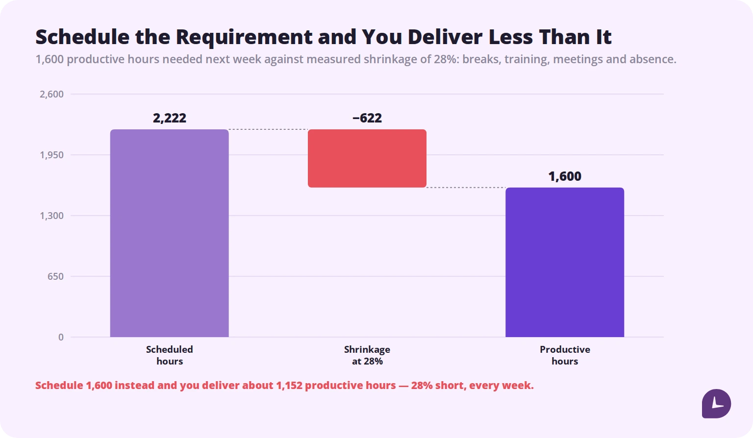
Worked example. You need 1,600 productive hours next week and your measured shrinkage is 28%:
1,600 ÷ 0.72 = 2,222 scheduled hours
Schedule 1,600 instead and you deliver about 1,152 productive hours, which is 28% short every week. Managers then describe the team as under-resourced, and the requested headcount increase is roughly the size of the shrinkage nobody measured.
Two rules. Measure your own shrinkage from recorded time rather than using an industry figure — the components differ enormously between operations. And split planned from unplanned: planned shrinkage such as training can be scheduled around, while unplanned shrinkage such as sickness needs buffer or relief cover.
Step 4: Set the labour budget
Coverage answers what you need. The budget answers what you can afford, and a schedule has to satisfy both.
For revenue-linked operations:
Labour budget = revenue forecast × target labour percentage
Budgeted hours = labour budget ÷ average loaded hourly cost
Worked example. A site forecasts $48,000 in revenue next week against a 28% labour target, with a loaded average cost of $19.50 an hour:
$48,000 × 0.28 = $13,440 → ÷ $19.50 = 689 hours
Use the loaded cost, not the wage. Payroll taxes, insurance and benefits typically add 20–30%, and budgeting on the base wage understates the cost of every hour. Our guide to labour costs covers the loaded rate.
When the coverage requirement and the budget disagree, that is information rather than an error. It means demand cannot be served at the target cost, and the decision is to accept a lower service level, change the mix of roles and rates, or revisit the target. Silently under-scheduling is the option most operations pick by default, and it produces the overtime that blows the same budget from a different direction.
Step 5: Build to intervals, not to days
A schedule can hit the correct total hours and still be wrong all day.
Two people from 07:00 to 15:00 and two from 14:00 to 22:00 is 32 hours, four people on the floor between 14:00 and 15:00, and two everywhere else. If the peak is at noon, that schedule is wrong at exactly the hour that matters.
Plan in 15 or 30-minute intervals for demand-driven work. Compare required against scheduled for each interval and you can see the gaps before publishing rather than discovering them in the shift.
Three techniques that fix interval gaps without adding hours:
Stagger start times. Shifts beginning on the hour create a coverage cliff. Offsetting by 30 or 60 minutes smooths the transition.
Schedule breaks against the demand curve. Breaks taken simultaneously during the peak remove coverage exactly when it is needed. This is a scheduling decision, not something to leave to the shift.
Use split or short shifts at the peaks where the law and the workforce allow it — noting that some states require a premium for split shifts.
Step 6: Apply the rules
Constraints are not a final check. They are inputs, because a schedule that violates them has to be rebuilt.
Overtime thresholds. Federal overtime is weekly over 40. California, Alaska, Nevada and Colorado apply daily thresholds, so four ten-hour days generates overtime in those states even at 40 hours. See our California overtime guide.
Rest and meal breaks. No federal requirement; many states have one. California requires a 30-minute meal period before the end of the fifth hour, and premiums are owed for non-compliant breaks.
Minimum rest between shifts. Clopening restrictions apply in most fair workweek jurisdictions, typically 10 or 11 hours.
Skills and certifications. A schedule that is numerically correct and puts an uncertified person on a task is not a schedule.
Availability and time off. Approved absence is a hard constraint, and building over it destroys trust in the published schedule faster than anything else.
Minor work restrictions, which vary by state and by school term.
Step 7: Publish, and publish early
In Oregon and ten US cities, covered employers must post schedules at least 14 days in advance and pay a premium for changes made inside that window. New York City’s retail ordinance is the outlier at 72 hours.
Coverage is not universal — the laws generally target retail, food service and hospitality with employer-size thresholds — but the operational lesson applies everywhere. Advance notice is the single thing hourly workers most consistently ask for, and short-notice scheduling is among the most reliable predictors of turnover.
Two practical points. Record the date you published, because that record is the evidence if notice is ever questioned. And note that paying predictability pay does not cure a notice violation; both obligations are enforced separately. Our daily schedule template includes a notice check, and the full jurisdiction list is in that guide.
Boost your business productivity
Track performance and streamline teamwork
Measuring whether it works
Six metrics, and the first two are the ones most operations never calculate.
| Metric | What it tells you | Target |
|---|---|---|
| Coverage variance by interval | Whether the schedule matches the demand curve | Within ±1 person in peak intervals |
| Forecast accuracy (MAPE) | Whether the forecast is worth scheduling against | Under 10% for stable operations |
| Labour cost vs budget | Scheduling accuracy against the financial plan | Within 3–5% |
| Overtime as a share of hours | Whether overtime is planned or reactive | Under 10% |
| Schedule adherence | Share of shifts worked as scheduled | 90%+ |
| Time to fill an open shift | Speed of the coverage process | Under 2 hours |
Read them together rather than individually. High overtime with good coverage means the forecast is low. Good adherence with poor coverage means the forecast is wrong rather than the team. High cost variance with accurate forecasting usually means shrinkage is unmeasured.
Measuring the forecast itself
Nobody in this field publishes this, and it is the foundation everything else rests on. A schedule built from a bad forecast cannot be fixed by better scheduling.
Mean absolute percentage error (MAPE) is the standard measure. For each interval, take the absolute difference between forecast and actual, divide by actual, then average across intervals.
Worked example across three intervals. Forecast 120, 140 and 95; actual 132, 131 and 110. The errors are 9.1%, 6.9% and 13.6%, giving a MAPE of 9.9%.
How to use it:
- Under 10% on stable, high-volume operations means the forecast is good enough to schedule against.
- 10–20% is typical for variable demand and means you need buffer.
- Over 20% means scheduling precisely against the forecast is false precision. Fix the forecast before optimising the schedule.
Track MAPE by day of week and by interval rather than as a single number. Most operations find that error is concentrated — a specific day, or the opening and closing intervals — and a targeted fix beats a general one.
Fairness, and why it shows up in your numbers
Fairness is usually framed as a culture issue. It appears in operational metrics.
Three things to track and equalise across the team:
Distribution of unpopular shifts. Nights, weekends, opens after closes. If the same people always draw them, that is visible to everyone and it drives attrition in the group you can least afford to lose.
Hours variance. Part-time staff whose hours swing between 12 and 34 a week cannot plan their income. Stability of hours matters as much as quantity for retention.
Time-off approval rates. If requests from one shift or team are approved less often, it will be noticed long before anyone raises it.
The connection to the numbers is direct: schedule instability raises turnover, turnover raises the share of new staff, and new staff lower the productivity rate that step two depends on. A scheduling practice that ignores fairness degrades its own inputs.
Common mistakes
Scheduling the required hours without adding shrinkage. Guarantees being 25–35% short.
Balancing daily totals rather than interval coverage. Right hours, wrong shape.
Forecasting hours instead of demand. Bakes last year’s staffing errors into this year’s schedule.
Budgeting on base wages. The loaded cost is 20–30% higher.
Treating constraints as a final check. They are inputs; a non-compliant schedule has to be rebuilt.
Staffing queue-based work linearly. Wait times deteriorate non-linearly with occupancy.
Never measuring forecast accuracy. Optimising a schedule against an unmeasured forecast is precision without accuracy.
Publishing late. Legally costly in eleven US jurisdictions and operationally costly everywhere.
How Monitask helps
Every number in this guide comes from recorded time. Productivity rate, shrinkage, adherence and cost variance are all measurements, and an operation that cannot produce them is scheduling on assumption.
Monitask records hours as they happen. Employees clock in when they start and clock out when they stop, so nothing runs in the background without their knowledge.

- Actual hours against scheduled hours give schedule adherence and coverage variance rather than an impression of them.
- Time by task and project separates primary work from meetings, training and admin, which is how shrinkage becomes a measured number instead of an industry guess.
- Attendance records quantify unplanned absence, the component of shrinkage that determines how much relief cover you need.
- Historical totals turn the productivity rate into your own figure rather than a benchmark from someone else’s operation.
See how it works: Monitask employee time clock software.
Sources
- US Department of Labor, Fact Sheet #23: Overtime Pay Requirements of the FLSA — the fixed workweek and 40-hour threshold.
- US Department of Labor, Wages and the Fair Labor Standards Act — absence of a federal meal or rest break requirement.
- Oregon Bureau of Labor and Industries — statewide predictive scheduling law with a 14-day advance notice requirement for covered employers.
- Erlang C, the standard queueing model for staffing randomly arriving, queued demand at a target service level.
Related reading
- Daily Schedule Template
- The Pitman Schedule
- Erlang C Calculator for Call Centers
- Choosing the Best Employee Scheduling Software
- What Is Schedule Adherence and Why It Matters
- The Importance of Proper Workforce Utilization
- California Overtime Law
FAQ
How is workforce scheduling different from workforce management?
Scheduling is the plan, built days or weeks ahead. Workforce management is the execution: attendance, real-time adjustments and payroll. Workforce planning is the longer horizon, deciding headcount and skills.
How do you calculate how many staff a shift needs?
Divide forecast demand for the interval by your productivity rate, then divide the result by one minus your shrinkage percentage. Queue-based work uses Erlang C rather than a linear division.
What is shrinkage in workforce scheduling?
The share of paid hours not spent on the primary work: breaks, training, meetings, admin and absence. It commonly runs 25–35%, and ignoring it means under-scheduling by that amount.
What interval should I schedule in?
15 or 30 minutes for demand-driven operations. Whole shifts only where coverage is fixed regardless of volume.
How do you set a labour budget for a schedule?
Multiply forecast revenue by your target labour percentage, then divide by the average loaded hourly cost to get budgeted hours. Use the loaded cost, which is typically 20–30% above the base wage.
How far in advance should schedules be published?
14 days. In Oregon and ten US cities it is legally required for covered employers, with predictability pay owed for later changes.
How do you measure whether scheduling is working?
Coverage variance by interval, forecast accuracy, labour cost against budget, overtime share, schedule adherence and time to fill an open shift. Read them together rather than individually.
What is a good forecast accuracy for scheduling?
Under 10% MAPE for stable, high-volume operations. 10–20% is typical with variable demand. Above 20%, fix the forecast before optimising the schedule.
Why do schedules with the right number of hours still fail?
Because hours and coverage are different constraints. The same total can be distributed so that the peak is understaffed and the quiet periods are overstaffed.